Graphs#
A graph is a pair \((V, E)\) consisting of a non-empty set of vertices \(V\) and a set of edges \(E\). \(E\) is a subset of the set \(\{\{u, v\} | u, v \in V\}\).
\(V\) can be any set of discrete elements. Often, it is a subset of the natural numbers. On the other hand, \(E\) is a set of subsets of \(V\). That is, \(E \subset \mathcal{P}(V)\).
Each of the elements of \(E\) have:
two elements, for example \(\{u, v\}\), where \(u, v \in V\), or;
one element, for example \(\{v, v\} = \{v\}\) for some vertex \(v \in V\).
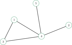
A graph of 5 vertices.#
In the figure above, we have a graph with 5 vertices and 5 edges.
Special Edges#
- Parallel edges
Two or more edges joining a pair of vertices.
- Loops
An edge that starts and ends at the same vertex.
The Language of Graphs#
Theories and Terminologies
A simple graph is what we have defined already as a graph. There is at most one edge between any two vertices.
A multigraph is what we call a graph which allows multiple edges between vertices.
A node or vertex is a discrete object of the graph.
The two vertices of an edge are called endpoints. That edge is said to join or connect the two vertices and the edge is incident to each of the vertices it joins.
When two vertices are joined by an edge, those vertices are called adjacent.
An edge which connects a vertex to itself is called a loop.
In some contexts, simple graphs do not allow loops.
A graph \(G = (V, E)\) of order \(n\) has \(|V| = n\).
The neighbourhood of a vertex \(v\), \(N(v)\), of a graph \(G = (V, E)\) is the set of all vertices adjacent to \(v\) in \(G\).
The degree of a vertex \(v\), \(deg(v)\), is the number of edges incident with it. Note that a loop contributes 2 to its degree.
Example
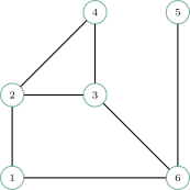
In this graph \(G\), we have:
The order of \(G\) is \(6\).
The degree of node \(3\) is \(3\).
The degree of node \(5\) is \(1\).
The degree of node \(6\) is \(3\).
The neighbourhood of node \(3\) is \(\{2, 4, 6\}\).
The neighbourhood of node \(6\) is \(\{1, 3, 5\}\).
Connectivity#
A path of a simple graph \(G = (V, E)\) is a sequence of vertices \((v_n)\) where an edge exists between \(v_i\) and \(v_{i + 1}\) for \(1 \leq i < n\).
Two vertices \(u, v\) in a graph are connected if there exists a path from \(u\) to \(v\). Otherwise, \(u\) and \(v\) are said to be disconnected. A graph is connected if every pair of vertices in the graph is connected.
Example
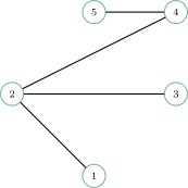
A connected graph.#
The above graph as many paths. And, in particular, every vertex is connected to every other vertex. Thus, the graph is a connected graph. In contrast, the graph below is disconnected.
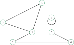
A disconnected graph.#
Complete Graphs#
A complete graph is a special kind of connected graph. Not only must the graph be connected—there must be a path from every vertex to every other vertex—but each path must be of length \(1\). That is, every vertex must be adjacent to every other vertex. A complete graph of order \(n\) is denoted \(K_n\).
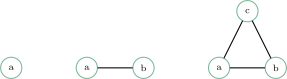
The complete graphs \(K_1\), \(K_2\), \(K_3\).#
A graph containing a single vertex is complete (vacuously so). A graph containing two vertices connected by a single edge is also complete. A graph of three connected into a triangle is also complete.
The first complete graphs are rather simple, but they quickly grow to be very complex.

\(K_4\)#
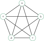
\(K_5\)#
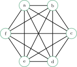
\(K_6\)#
Why are these so complex? Precisely because of the definition of a complete graph. There must be an edge between every pair of verices. Of course, we can count how many edges there will be.
A complete graph of order \(n\) has \(\frac{n(n-1)}{2}\) edges.
Proof
A complete graph has an edge between any two vertices. For a graph with \(n\) vertices, if we choose any two vertices, there must be an edge between them. There are \(\binom{n}{2}\) such choices.
Special Graphs#
We have already seen complete graphs as a special graph with a special name. There are many other useful graphs with special names and different properties.
Cycles#
A cycle graph is a graph with exactly one cycle. The cycle graph of order \(n\) is denoted \(C_n\).
As a consequence of cycles, a cycle graph must have 3 or more vertices.

\(C_3\)#

\(C_4\)#
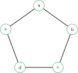
\(C_5\)#
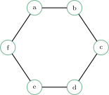
\(C_6\)#
Wheels#
A wheel graph is a cycle graph in which one extra vertex has been added which connects to every other vertex in the cycle. The wheel graph of order \(n\) is denoted \(W_n\).
We call these “wheels” because they look like a wheel: a central hub and a tire or rim. The single vertex connected to every other is the “hub”, the cycle is the “rim”.
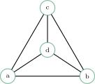
\(W_4\)#

\(W_5\)#
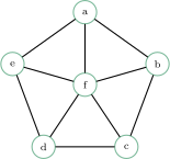
\(W_6\)#
Notice that \(W_n\) is \(C_{n - 1}\) with the added hub vertex. Moreover, notice that \(W_4\) is the same as \(K_4\).
Planar Graphs#
A planar graph is a graph that can be drawn with no overlapping edges.
Every cycle graph is planar. Every wheel graph is planar. In contrast, every complete graph of order \(5\) or higher is not planar.
\(W_6\) is planar.#
\(C_6\) is planar.#
\(K_4\) is planar, even if it does not look like it.#
Important
Just because planar graphs can be drawn with overlapping edges, does not mean that they are necessarily not planar.
\(K_4\) is planar even though its typical way of drawing has crossed edges. Indeed, \(K_4\) and \(W_4\) are the same graph, and \(W_4\) is obviously planar.
\(K_4\) is planar.#
\(W_4\) is planar.#
So, a graph is planar if there is at least one way of drawing it so that there are no crossed edges.
Bipartite Graphs#
A bipartite graph is a graph \(G = (V, E)\) whose vertices can be partitioned into two disjoint sets \(V_1\) and \(V_2\) such that every edge in \(E\) has one endpoint in \(V_1\) and one endpoint in \(V_2\).
In a bipartite graph with vertices partitioned into \(V_1\) and \(V_2\), there cannot be any edges within a partition.

\(C_4\) is a bipartite graph.#
\(C_4\) is a bipartite graph because its vertices can be partitioned into two groups so that there are no edges within either partition. In the case of \(C_4\), opposite corners are in the same partition, as indicated by the coloring above.
Bipartite graphs are highly related to the problem of graph coloring. Graph coloring is just some way of labeling or grouping vertices. Since graphs are highly visual, we usually use colors. But, “coloring” can mean any form of labeling of vertices.
Tip
A graph is bipartite if its vertices can be colored using exactly two colors so that now two adjacent vertices have the same color.
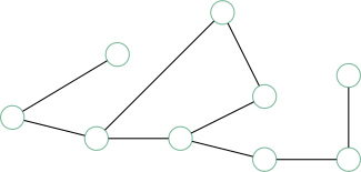
A bipartite graph \(G\).#
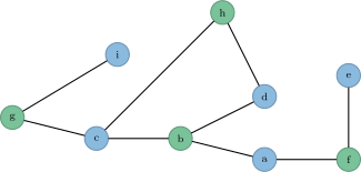
A coloring of \(G\) with two colors.#
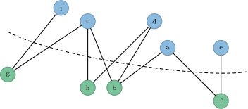
Moving the vertices to explicitly show edges between colors.#
Tip
A simple graph is a bipartite graph if and only if it does not contain any cycles of odd length.
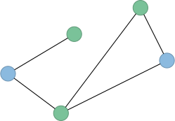
A graph with a cycle of length \(3\) cannot be bipartite.#
Complete Bipartite Graphs#
A complete bipartite graph is a bipartite graph whose vertices can be partitioned into two sets \(V_1\) and \(V_2\) and there is an edge for every vertex in \(V_1\) to every vertex in \(V_2\). Where \(|V_1| = m\) and \(|V_2| = n\), the complete bipartite graph is denoted \(K_{m, n}\).
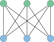
\(K_{3, 3}\)#
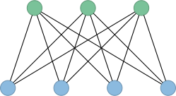
\(K_{3, 4}\)#
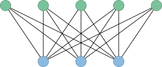
\(K_{5, 3}\)#
Weighted Graph#
A graph where each edge is assigned a numerical label or “weight”.
Trees#
A tree is a simple connected graph with no cycles.
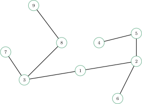
A tree with 9 vertices.#
Rooted Trees and Children#
A rooted tree is a tree in which one of the vertices has been designated as the root.
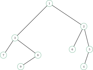
A tree rooted at node \(1\).#
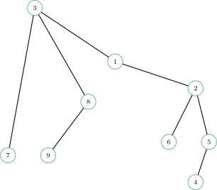
A tree rooted at node \(3\).#
Designating a root in a tree includes special relationships between vertices. It derives from the fact that there is a unique simple path from any vertex to any other vertex in a tree. The terminology used most commonly is based on ancestry.
The root is the “oldest” ancestor.
Each of the children of the root are the vertices which have a path of length \(1\) from the root.
The children of those children are vertices which have a path of length \(2\) from the root.
Conversely, the children of the root tree have the root as their parent.
To speak about a vertex’s children and children’s children, etc. we say descendants.
Visually, rooted trees are almost always drwan with the root at the top. Then, children are always drawn lower than their parents.
If we wanted to be very precise with the drawing of a rooted tree, we would draw every child at the same level of a tree at the same y-position. The level of a vertex in a tree is its distance from the root.
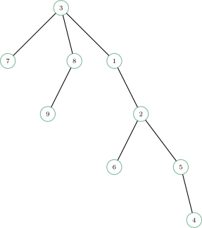
A “properly drawn” tree rooted at node \(3\).#
A very important property of tree is that they admit a recursive description. For every non-root vertex \(v\) in a tree, there is a subtree rooted at \(v\).
Given a non-root vertex \(v\) of a rooted tree, the subtree rooted at \(v\) is the subgraph rooted at \(v\) and induced by \(v\) and all its descendants.
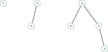
Three subtrees of the previous tree figure: the subtree rooted at node \(7\), the subtree rooted at node \(8\), and the subtree rooted at node \(2\).#
Binary Trees#
A binary tree is a rooted tree where each vertex has at most 2 children. A full binary tree is a binary tree where every vertex has exactly 2 children or 0 children.
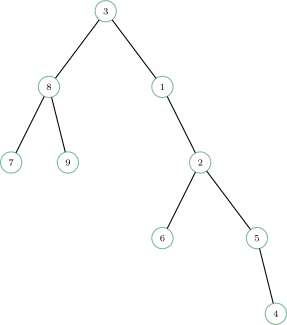
A binary tree.#
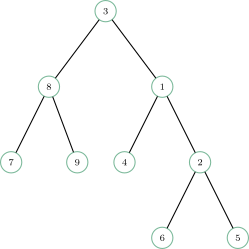
A full binary tree.#